
The simple analytics of changes in net farm income
In writing column 1004 (https://tinyurl.com/ruksgn6) which focused on changes in state-level net farm income we noticed that the Economic Research Service of the United States Department of Agricultural (USDA/ERS) had extended their data extraction tool back to 1929 and provides data in nominal dollars (the prices farmers saw at the time) as well as real dollars (inflation adjusted dollars).
We usually present data in nominal dollars because nominal dollars are more relatable than inflation adjusted dollars. But inflation adjusted dollars provide an important comparison standard for analysis and for tracking information across time. In fact, in the case of net farm income, inflation adjusted data do a remarkable job of contrasting agriculture’s good times from the not-as-good times.
Clearly during the 9 decades between 1929 and 2019, agriculture enjoyed 3 periods of exceptional prosperity (Fig. 1). Very different circumstances underlie these income explosions, yet analytically they are very similar. In each case, the reasons were not mammoth changes in population or income, or multi-year drastic shortfalls in agricultural production, or the other supply and demand elements that economists usually talk about.
No, in each case the primary cause was a huge increase in the agricultural demand brought on by government action of some sort, either by our federal government or “governments” elsewhere.
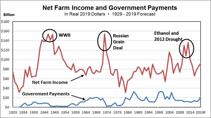
Figure 1. Net Farm Income and government payments in real 2019 dollars, 1929-2019 Forecast. Source: USDA/ERS Farm Income and Wealth Statistics (https://tinyurl.com/vafwly8).
The first agricultural income peak occurred during WWII when the US was supplying foodstuffs for US European allies and US combat troops fighting to obtain a victory against Axis troops in various theatres of operation (Europe, Asia, and North Africa).
The second peak, sharper and shorter than the first, was triggered primarily by the entry of the Soviet Union into the world grain market in response to a significant production shortfall in grains.
The third peak was the period of increasing demand for corn as a result of the adoption of the Renewable Fuels Standard (RFS) in 2005. (This peak was extended by short crops in 2010 and 2011 and a full-blown crop failure across much of the corn belt in 2012.)
Based on what we know about the 1910 to 1929 period, if USDA/ERS net farm income data were available, a fourth peak in agricultural income would also be evident, triggered by WWI and the provision of foodstuffs to Europe.
Each of the income peaks occurred because of a sharp increase in exogenous or outside demand. In each case there is a sequence of market reactions and consequences that follow a distinct pattern.
Farmers cannot expand the within-year crop production by “adding shifts” like in a manufacturing facility so the price of grains tripled or quadrupled.
Next euphoria and fear set in. Farmers become euphoric believing that a new era of permanently-high agricultural prices has finally arrived. They respond by heavily investing in machinery and by bidding up the price on inputs, especially land.
Others express fear that agriculture cannot keep up with future growth in food demand. This fear sets off a campaign by public officials, input suppliers and agricultural researchers to convince the public of the coming food “shortages” and to promote a massive expansion of agricultural research and technological innovation.
Reinforced by the talk of future shortages, farmers redouble their efforts to increase production and productive capacity.
But the good times do not last. Each time the government-induced growth in agricultural demand either quits growing (as in the ethanol case) or disappears (as in the international cases).
Agriculture is then saddled with a productive capacity that exceeds agricultural demand at a profitable price.
Agriculture is good at redistributing production among crops, but it is horrible at reducing crop production in total. Since individual farmers provide only a miniscule proportion of total production, they cannot affect commodity prices. From their perspective reducing production can only reduce revenue. Over time with markedly low prices, production does decline but by relatively little.
Just as the total supply of agricultural products is, as economists keep saying, price inelastic, so is the demand for food and agricultural products in general—a price decline does not expand the quantity demanded very much.
Besides these periodic disruptions, add the fact that as a rule, US agricultural productivity tends to increase faster than total demand and you have an in-the-nut-shell version of why agriculture tends to have chronic price and income problems.
Policy Pennings Column 1008
Originally published in MidAmerica Farmer Grower, Vol. 37, No. 254, December 27, 2019
Dr. Harwood D. Schaffer: Adjunct Research Assistant Professor, Sociology Department, University of Tennessee and Director, Agricultural Policy Analysis Center. Dr. Daryll E. Ray: Emeritus Professor, Institute of Agriculture, University of Tennessee and Retired Director, Agricultural Policy Analysis Center.
Email: hdschaffer@utk.edu and dray@utk.edu; http://www.agpolicy.org.
Reproduction Permission Granted with: 1) Full attribution to Harwood D. Schaffer and Daryll E. Ray, Agricultural Policy Analysis Center, Knoxville, TN; 2) An email sent to hdschaffer@utk.edu indicating how often you intend on running the column and your total circulation. Also, please send one copy of the first issue with the column in it to Harwood Schaffer, Agricultural Policy Analysis Center, 1708 Capistrano Dr. Knoxville, TN 37922.